Semantic Segmentation

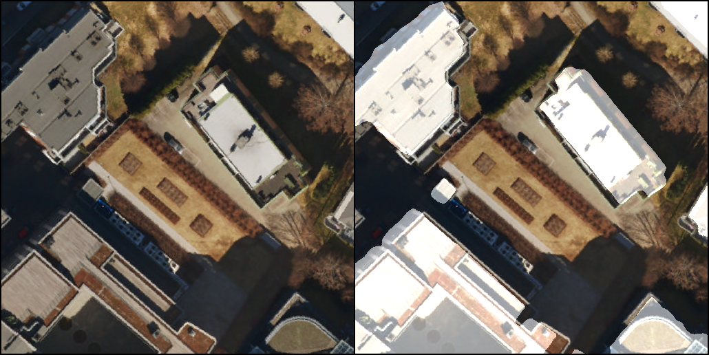
The goal of semantic image segmentation is to classify each pixel of an input image with a corresponding class of what is being represented. Because we’re predicting for every pixel in the image, this task is commonly referred to as dense prediction. The expected output in semantic segmentation is a complete high resolution image in which all the pixels are classified.

Convolutional Neural Networks

A Convolutional Neural Network (CNN), in short, is a deep learning algorithm commonly used to, assign importance and differentiate between various objects and aspects of an image fed into it. It does so by changing and updating inherent weights and biases, based on a ground truth via supervised learning.

To some extent, they are very similar to regular neural networks that use Multilayer perceptrons(MLPs), both are made up of learnable weights. But contrary to MLPs, CNNs have an architecture that explicitly assumes its inputs have structures like images. This allows encoding said property into the architecture, by sharing the weights for each location in the image and having neurons respond only locally. I.e a CNN is composed of convolutional layers without any fully-connected layers or MLPs usually found at the end. This provides efficiency for the forward pass implementation, and most importantly reduces the number of parameters in the network compared to a fully connected network(FCN). E.g if a 3-channel image of size 256 by 256 pixels were to be feed into an FCN, it would require the first hidden layer to have 196608 input weights.

The pre-processing required in a CNN is also much lower as compared to other classification algorithms. While in primitive methods filters are hand-engineered, with enough training, CNNs can learn these filters. The architecture of a CNN is analogous to that of the connectivity pattern of Neurons in the Human Brain and was inspired by the organization of the Visual Cortex. Individual neurons respond to stimuli only in a restricted region of the visual field known as the Receptive Field. A collection of such fields overlap to cover the entire visual area. In particular, a node in a layer is only connected to a small region of the previous layer, contrary to each node in the layer before in a FCN. As mentioned, this reduces the number of parameters vastly.

Forward propagation

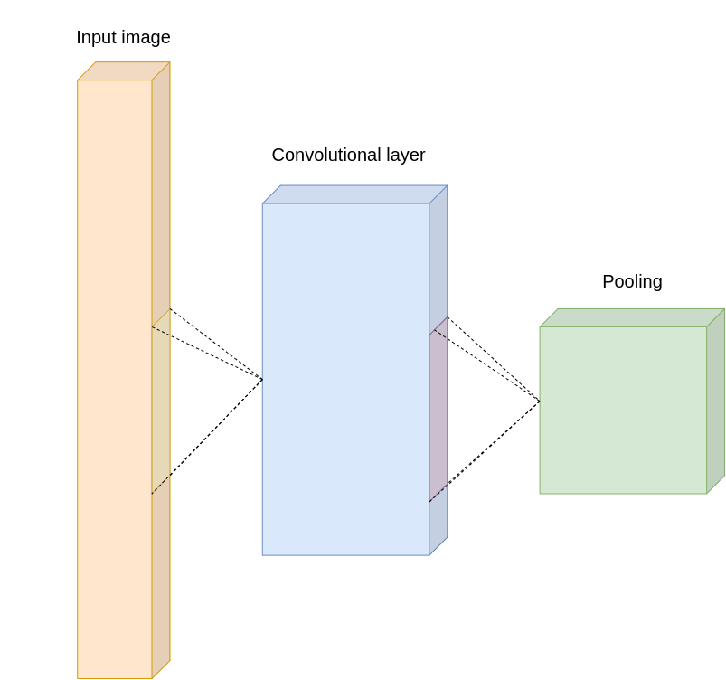
Forward propagation in a CNN architecture consists mostly of convolutional layers, pooling layers, and activation functions.

Convolution is the first layer to extract features from an input image or a previous layer. Convolution preserves the relationship between pixels by learning image features using small filters, also known as kernels, passing them over the image. I.e layer values from small areas in the previous layer or input images are used to calculate new values in the current layer. The small area is covered by a kernel of trainable weights, and the use of a compact area allows the new value in the current layer to retain surrounding information from that area in the former layer.

Pooling layers offer an approach to downsample areas, known as feature maps, by summarizing the presence of the different values in patches of the feature map. Two common pooling methods are average pooling and max pooling that summarize the average presence of a feature and the most activated presence of a feature respectively. In short, it is an operation whose objective is to reduce spatial size of the input by selecting a certain value and discarding the rest.

Activation functions are usually somewhat simple functions implemented at the end of a layer. They are highly important as they introduce non-linearity to the networks, which allow the layer and neurons to learn and pass answers down the pipeline.

Commonly, the last layers of CNNs are fully connected layers to make predictions. However, in this work, other modules are used in the aft parts of the architecture. For this reason, there are no further mentions of FCNs. The output layer is generally a Softmax layer to clamp the class scores to a value between 0 and 1. The aforementioned layers are described in this subsection.

Convolutional layer

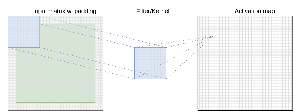
Convolutional layers are the most important building blocks used in CNNs, hence their name[1]. In the context of a CNN, convolution is a linear operation that involves the multiplication of a set of weights with the input, much like a traditional neural network. Given that the technique was designed for two-dimensional input, the multiplication is performed between an array of input data and a two-dimensional array of weights, called a filter or a kernel.

The filter is smaller than the input data, also the type of multiplication applied between a filter-sized patch of the input and the filter is a dot product. This multiplication produces a single scalar, resulting in a two-dimensional activation map. The spatial size of this activation map depends on whether the input was padded or not. Padding refers to the number of pixels added to an image when it is being processed by the kernel. Adding padding to an image processed by a CNN allows for a more accurate analysis of images, and allow the spatial size of the resulting activation map to be the same as the input.

Pooling Layer

Pooling is a common feature imbibed into CNN architectures, and the main idea behind these layers is to sum-up features from maps generated by previous convolution layers[1]. Formally its function is to reduce the spatial size of the activation maps, such that it reduces the number of parameters and hence computation in the network.

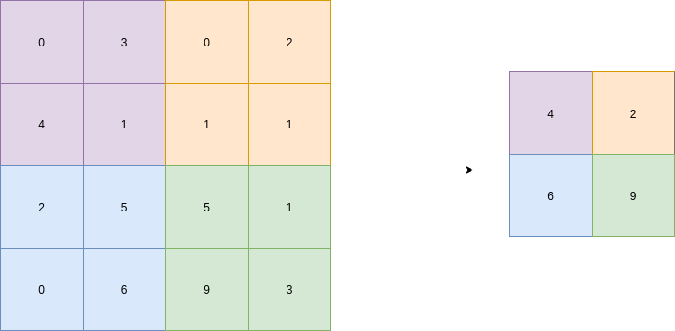
The most common form is max pooling. In a relatively simple operation, a kernel of the chosen size is applied as a sliding window across each activation map individually. The largest value within the area the kernel is applied to in the activation map is then chosen as the representative for that area. The kernel size and the stride are hyperparameters chosen by the designer of the architecture. The stride tells of how many pixels the kernel jump after each application. If the stride is equal to the number of rows in the kernel, none of the areas the kernel is applied to will overlap. In a max-pool layer, this is the most common approach.

Max pooling is done in part to help over-fitting by providing an abstracted form of the activation maps. As well as it reduces the computational cost by reducing the number of parameters to learn, and it also provides basic translation invariance to the internal representations. Max pooling is done by applying a max filter over non-overlapping subregions of the initial activation maps.

The idea is to retain the information which best describes the context of the image, from each region and throw away the information which is not important.

Rectified Linear Unit

The Rectified Linear Unit(ReLu) is a non-linear activation function that is used in multi-layer neural networks or deep neural networks. For input values of x the function can be represented as:

$$ \begin{align*} f(x) = max(0,x) \end{align*} $$

(1)

According to equation 1, the output of ReLu is the maximum value between zero and the input value. The output is equal to zero when the input value is negative and the input value when the input is positive. I.e

$$ \begin{align*} f(x) = \begin{cases} x, \mbox{if } x \geq 0\\ 0, \mbox{otherwise} \end{cases} \end{align*} $$

(2)

Traditionally, some prevalent non-linear activation functions, like sigmoid functions and hyperbolic tangent, have been used in neural networks to get activation values for each neuron. However, the ReLu function has become a more popular activation function because it can accelerate the training speed of deep neural networks compared to traditional activation functions. This because the derivative of ReLu is 1 for positive input. Owing to a constant, deep neural networks do not need to take additional time for computing error terms during the training phase.

The ReLu function does not trigger the vanishing gradient problem when the number of layers grows. This is because the function does not have an asymptotic upper and lower bound. Thus, the earliest layer (the first hidden layer) can receive the errors coming from the last layers to adjust all weights between layers. By contrast, a traditional activation function like sigmoid is restricted between 0 and 1, so the errors become small for the first hidden layer. The mentioned scenario will lead to a poorly trained neural network.

Normalization Layer

One of the most common Normalization techniques used nowadays is Batch Normalization (BN). It is a strategy that normalizes interlayer outputs in a neural network. This in effect resets the distribution of the output from previous layers to be more efficiently processed by the subsequent layers[2].

It relieves numerous problems with properly initializing neural networks. In practice, networks that use BN are significantly more robust to bad initialization. Additionally, BN can be interpreted as doing preprocessing at every layer of the network, but integrated into the network itself in a differentiable manner[3].

The method leads to faster learning rates, as normalization ensures that there are no extreme activation values. It also allows each layer to learn independently from others, and it reduces the amount of data lost between the processing layer. This improves learning accuracy throughout the network. Ioeffe and Szegezy [4] report a state of the art classification model that achieved the same accuracy but requiring 14 times fewer learning iterations to do so using BN.

However, according to Wu et al. [5] using batch sizes (BS) less than 32 with BN results in a dramatically increased model error. There are situations that one has to settle for sizes of BS less than 32. I.e when memory consumption of each data sample is too high, with large networks or simply with lacking hardware requirements. This work does handle somewhat high-resolution images, and for this reason, alternatives to BN which work well with small batch size are needed. Group Normalization (GN), proposed by Wu et al. is one of the latest normalization methods that avoids exploiting the batch dimension, thus is independent of batch size. They report that with a ResNet-50 model trained in the ImageNet training set using 8 GPUs, a reduction in BS from 32 to 2 resulted in little to no change in error with GN contrary to an increase in error when using BN.

Softmax layer

In many neural networks, the last layer is often a softmax layer[2]. It is used to transform values of the class scores to numbers ranging from 0 to 1. The sum of the class-wise predictions is 1, so the layer can be interpreted as a probability spread function and looks like this:

$$f_j(\mathbf{z}) = \frac{e^{z_j}}{\sum_ke^{z_k}}$$

(3) where z is the set of scores to be squashed. As one can see, the formula takes each class score in the power of e, and divides it by the sum of the entire set in the power of e.

Backpropagation

Backpropagation, short for backward propagation of errors is arguably the most important part of the training process. This is where the learnable parameters, weights, and biases in the network are updated to make improved predictions [6]. When a network is run through the training loop, a loss function is calculated, which represents the network’s predictions and its distance from the true labels. Backpropagation allows us to calculate the gradient of the loss function, proceeding backward throughout the network from the last layer to the first. For the gradient to be calculated at a particular layer, the gradients of all following layers are combined via the chain rule of calculus. This enables each weight to be updated individually to, gradually reduce the loss function over many training iterations. Loss functions are described in more detail further down in this section.

The loss function provides the loss, or error, L at each output node, and the objective is to minimize this value. The input to this function is x and consists of the input values in the training data and the learnable parameters in the network. The input data is static and cannot be altered to minimize L, but the parameters are. The backpropagation method calculates how much the parameters should be altered, by finding their gradients relative to the error output from the loss function. Said gradient is calculated by taking the partial derivatives of the output with respect to input values. E.g if an output depends on three input values, the output has three partial derivatives. The gradient itself is the vector consisting of all these partial derivative values.

To attain the gradient, partial derivatives between each parameter relative to the error output that the particular parameter contributed to must be calculated. For this to be possible, the process must start at the output layer. Every node obtains input values from a set of nodes in the previous layer. In the forward pass, each node calculates its output values based on the input and the gradient of the input values relative to its output value. During backpropagation, moving backward from the output layer to the input layer. All the nodes in time learn the gradient of its output value relative relative to output of the value it contributed to calculating. Per the chain rule, the aforementioned gradient should then be multiplied with all the local gradients that the node has obtained. The process hence repeats when the input nodes to the particular node know the gradient of its output relative to the final error output value. In this manner, the gradient for every parameter from the output to the input layer will know its gradient relative to the final error output value of which they contributed to, and can be modified to minimize said error based on the gradient value.

Loss functions

The loss function is used to determine the error or in other words the loss, between a network prediction and a given target value. It expresses how far off the network is at doing a correct prediction. It is usually expressed as a scalar that increases by how far off the model is. As the goal of the model is to perform correct predictions, the main objective of the training process is to minimize this error.

A common loss function is the cross-entropy loss function. Cross-entropy loss, or log loss, measures the performance of a classification model whose output is a probability value between 0 and 1. The function can be described as:

$$ -\sum^M_{c=1}y_{o,c}\log(p_{o,c}) $$

(4)

where M is the number of classes, y is the binary indicator if class label c is the correct prediction for the observation o and p is the predicted probability observation o With binary classification, where the number of classes M equals 2, the cross-entropy can be calculated as:

$$ \begin{align*} -(y\log(p)+1-y)\log(1-p)) \end{align*} $$

(5)

If M > 2 we calculate a separate loss for each class label per observation and sum the result.

In practice, this gives a high loss value to wrong predictions and a 0 loss value to the right predictions. This is the behavior that is wanted in a loss function since when minimized it will give better predictions. This is the base of the loss function used in this work.

Fully Convolutional Network

The goal of semantic image segmentation is to classify each pixel of an input image with a corresponding class of what is being represented. Because we’re predicting for every pixel in the image, this task is commonly referred to as dense prediction. The expected output in semantic segmentation is a complete high-resolution image in which all the pixels are classified.

In a typical convolutional network, the height and width of the input gradually reduce i.e downsampling, because of pooling. This helps the filters in the deeper layers to focus on a larger receptive field. However the depth, number of filters used, gradually increase which aids in extracting more complex features from the image. From the pooling layers, one can somewhat conclude that by downsampling, the model better understands the context presented in the image, but it loses the information of locality, i.e where said context is located. Thus if one were to use a regular convolutional network with pooling layers and dense layers, the locality information will be lost and one only retains the contextual information.

A Fully Convolutional Network(FCN) is a CNNs based network that progresses from coarse to fine inference to predict every pixel like semantic segmentation requires[7].

Deconvolution

To get an output that is expected in semantic segmentation, there is a need to convert, or upsample, the low-resolution information provided by a typical CNN to high resolution, and recover the locality information.

Deconvolution, sometimes also called Transposed Convolution or fractionally strided convolution, is such a technique to perform upsampling of an image with learnable parameters[8]. On a high level, transposed convolution is exactly the opposite process of a normal convolution i.e., the input volume is a low resolution image and the output volume is a high-resolution image. A normal convolution can be described as a matrix multiplication of input image and filter to produce the output image. In short, by taking the transpose of the filter matrix, it is possible to reverse the convolution process, hence the name transposed convolution.

---

• ← Previous Post
• Next Post →